Searching for “mountain” in your Apple/Google photos library, browsing the Related Pins section in Pinterest, or using Google Lens to find information about the world around you - these are all instances of content-based search. With the increasing ubiquity of cameras, more and more of the data we create is visual: 400 hours worth of videos are uploaded to Youtube every minute, 80 million photos are shared on Instagram on an average day. A growing number of cultural institutions are digitising parts of their collections: Metropolitan Museum of Art (375,000 items), British Library (a million items), and just recently the Smithsonian Design Museum has opened access to over 200,000 items. With this abundance of visual data, it’s obvious that our tools for content discovery and search need to evolve. In this post we’ll work through a simple implementation of content-based search that leverages a state-of-the-art pre-trained convolutional neural network and approximate nearest neighbour search to create a simple but powerful search system.
We will be using PyTorch and the fast.ai library to create the search system. The fast.ai library is an abstraction that sits on top of PyTorch, providing a set of utility and convenience methods to quickly prototype and iterate on deep learning models. Although the library is extremely useful, documentation is non-existent and support very minimal. The best way to get started with the library is to work your way through the fast.ai deep learning course, or if you’re familiar enough with PyTorch and deep learning then jump straight into their example notebooks. Of course, all of this can be done using purely PyTorch, Keras, or any other framework.
Visually Similar Artworks
We’ve created a simple demo to show how the system performs with finding visually similar artworks. You can search by selecting an artwork from the image-drawer at the bottom. The system will find and show artworks that are the ‘closest’ (content and style) to the selected artwork from within our collection. Our collection, sourced from WikiArt, contains a total of 10,000 artworks from 28 different styles. All artworks are either in the public domain or have fair use copyright policy.
Tips for interaction:
- You can also select an artwork from “Similar Artworks” to perform a search; we encourage the rabbit hole.
- Switch between network architectures to see how results differ.
- Hit “refresh choices” to get a fresh new batch of artworks to pick from.
- Hover over artworks to find out the artist and the name of the work.
Note: Due to server limitations, we’ve pre-computed the search results for this demo. Important to note that it’s not a limitation of the search being slow.
Overview of Approach
Creating an Image Representation
How do we create a highly compressed representation that encodes both the high-level content and the overall style of the image? One approach would be to train a Variational Autoencoder or a Generative Adversarial Network, and then use the learnt latent representation. That would be a fun project, but there is no need to start from nothing. We have access to state-of-the-art pre-trained deep convolutional neural networks (DCNNs), and although the networks were trained mainly to classify dog-breeds (ImageNet), they work as excellent generic feature extractors.
This property of DCNNs was very well demonstrated by Gatys et al. with style transfer. The original paper used a pre-trained VGG-16 network to extract the style of any painting and apply it to any photo. From the paper:
When Convolutional Neural Networks are trained on object recognition, they develop a representation of the image that makes object information increasingly explicit along the processing hierarchy. … Higher layers in the network capture the high-level content in terms of objects and their arrangement in the input image but do not constrain the exact pixel values of the reconstruction.
There are many ways to construct a feature representation of an image from DCNNs. It’s common to use multiple layers of the network to construct a feature representation. Pinterest detail that they use layers fc6 and fc8 from the VGG network as part of their image representation pipeline. For our case, we’re going to keep it simple and use the final feature layer (right before the output layer) as the compressed representation. This is a nice graph that comapres different model architectures on their classification accuracy vs number of operations:
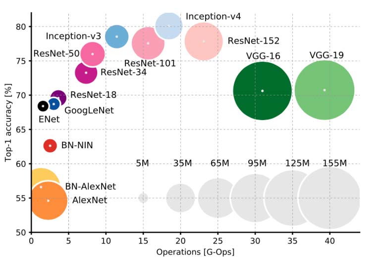 |
|---|
| Source: An Analysis of Deep Neural Network Models for Practical Applications |
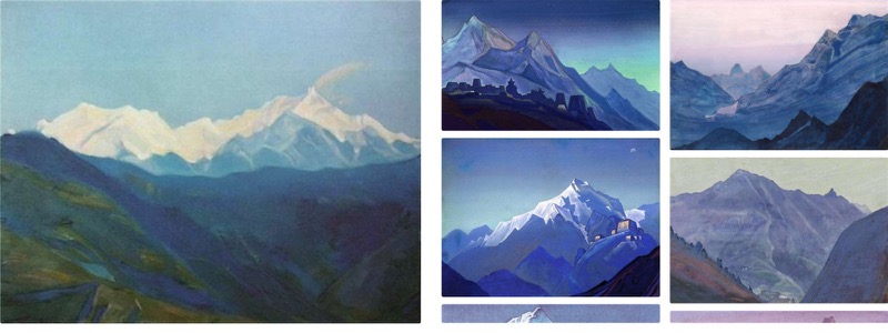
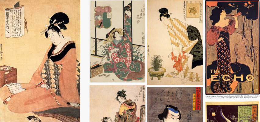
As it’s impractical to build a visual-similarity test set, we can’t cross-validate between all the different networks to pick the best performing. We performed an empirical evaluation of three networks: Inception-V4 (1536 feature dimensions), ResNet-50 (2048 feature dimensions), and VGG-16 (2048 feature dimensions). Our testing showed that although Inception-V4 was generally the best at surfacing results with similar content, it didn’t perform too well in surfacing images of similar style. VGG-16 had the inverse problem of being too sensitive to style and disregarding the content. We found ResNet-50 to have the best balance of both style and content out of the three networks. You can compare the three networks yourself in the demo above.
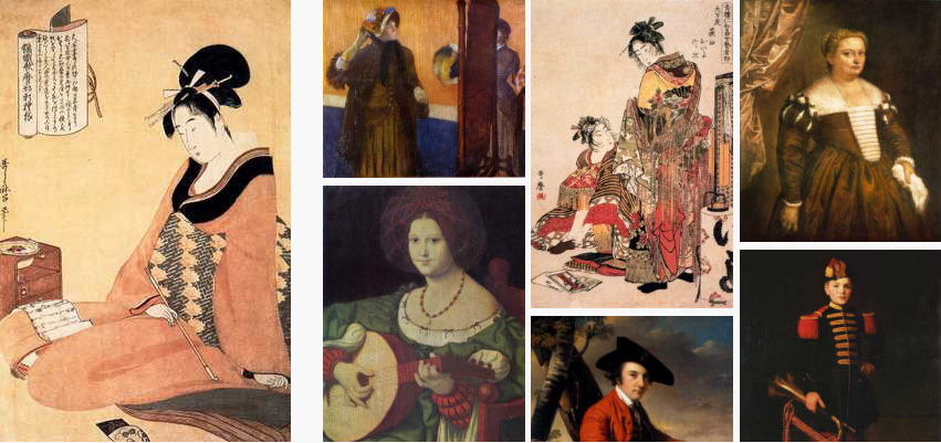 |
|---|
| Inception-V4 results for “Reading a Letter” by Kitagawa Utamaro |
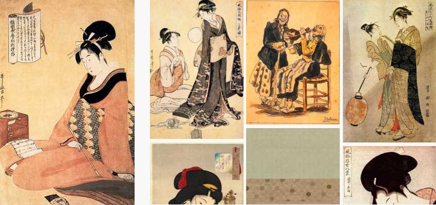 |
|---|
| ResNet-50 results for “Reading a Letter” by Kitagawa Utamaro |
 |
|---|
| VGG-16 results for “Reading a Letter” by Kitagawa Utamaro |
As our focus is to build content-based similarity search, we’ll use Inception-V4 for the tutorial.
Fast Nearest Neighbour Search
We are dealing with 10,000 artworks and at least 1536 dimensions, now we need a data structure suited for performing fast neighbourhood lookups. It’s possible to precompute a distance matrix (O(n^2) time complexity) with a small dataset, but this poses severe limitations with large and/or dynamic datasets. We could get away with pre-computing distances for our example, but let’s assume pre-computation is not allowed. Given the the number of items and dimensions we are working with, there is no real-time and time-efficient algorithm that we can use to perform exact nearest neighbour searches. To get real-time search results we must make a tradeoff with finding approximate nearest neighbours (ANN).
Approximate nearest neighbour Python libraries is a surprisingly crowded field. We’ll be using Annoy because it’s well documented and extremely simple to use. Annoy is middle of the road when it comes to query speed, the creator (Erik Bernhardsson) also maintains ANN-Benchmarks where he compares various ANN search libraries.
I won’t be going into how Annoy works, but if you’re curious, I recommend reading Erik’s great post on the algorithms and data structures behind it.
Implementing the System
Here is the Github repository for easy reference.
Environment Setup
Let’s install all the packages we’re going to use first. I recommend using a virtual environment because the fast.ai library is not yet compatible with the latest PyTorch, so it may uninstall your current version and cause all kind of conflicts with current projects. If you prefer to use Anaconda to manage your environments, follow installation instructions from the fast.ai Github.
1 | $ pip install git+https://github.com/fastai/fastai.git |
Image Dataset
PyTorch provides a very nice way to represent a custom dataset using the torch.utils.data.Dataset class. We save all image paths on initialisation, and load each image only when it’s requested (__getitem__ method).
We’re passing in an extra parameter tfms (read transforms) to the class, these are simply a set of transformations that need to be applied to the image before it’s returned. They’re necessary especially when using pre-trained models as most require some form of image normalisation.
1 | from fastai import conv_learner as learner |
Feature Computation
Before we setup our Inception-V4 model, we need a little utility to capture and store the output of a layer once a forward pass has been completed. PyTorch provides the ability to register a ‘hook’, which is automatically called when a forward pass is executed on a PyTorch Variable.
1 | class LayerHook(): |
Now we can setup the Inception-V4 model, and register a hook onto the final feature layer. Different pre-trained models are represented differently, some as flat lists, other as nested lists. To pick the feature layer it’s necessary to break down and explore the model structure:
print(learner.children(model)): prints the entire network structure layer by layer.from torchsummary import summary: prints a table that contains the type, the output shape, and the number of parameters in the each layer.
That’s how we arrive at the magic [-2][-1] indices for referencing the feature layer.
1 | from torchsummary import summary |
Now that we have the dataset and the model, we can write a method to loop over all the images and return the computed features.
1 | from torch.utils.data import DataLoader |
NO_CROP: resizes image into square dimensions regardless of the original aspect ratioCENTER_CROP: reduces the smallest dimension of the image to the specified size (maintaining aspect ratio), then center crops to create a square image
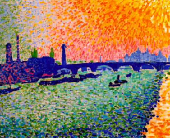
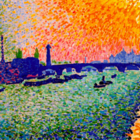
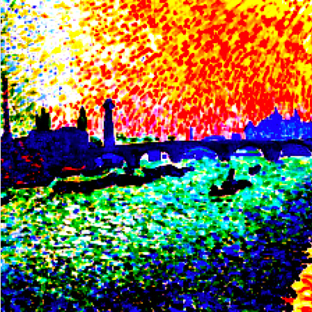
There is an additional helper method (visualise_transforms) in the Github repository that allows you to visualise how the image changes after each transform is applied. Here is that process:
 |
 |
 |
|---|---|---|
| Original (“The Bridge” by Andre Derain) | Center cropped | Normalised |
Let’s load up the dataset and compute the features!
1 | dataset = ImageDataset('data/art_collection/', tfms) |
Approximate Nearest Neighbour Search
Annoy has been built with the intention of simplicity so this leaves very little room for parameter tweaking. The only two choices we have are:
metric: the distance metric to use, choices are: “angular”, “euclidean”, “manhattan”, “hamming”, or “dot”num_trees: the number of trees to use in the forest, higher number gives higher precision but at cost of speed.
In our tests we found that the cosine (“angular”) distance metric and 25 trees gave pretty good results.
1 | from annoy import AnnoyIndex |
Performing a Search
We can put everything together and perform our first search.
1 | query_index = np.random.randint(0, ann.get_n_items()) |
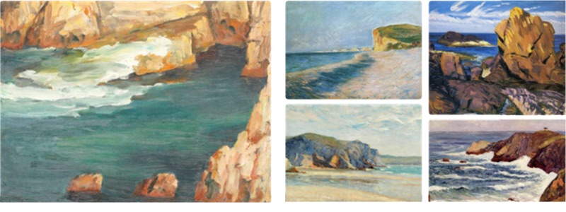 |
|---|
| Query (“Cape Caliacra” by Stefan Popescu) and results |
Pretty neat, right?
You can use any image (doesn’t have to be from your dataset) and find images similar to it in your corpus. First compute a feature representation of the image using your model, and then use the ann.get_nns_by_vector method to perform your search.
By leveraging a state-of-the-art pre-trained convolutional neural network, and the great open-source community around Python we’ve built a fairly complex visual search system. We’ll definitely be expanding on this system and making the search functionality more powerful. The next step is to look at how we can perform searches with required attributes, e.g. find visually similar images in the style of Pointillism (or any other attribute). We’ll keep you updated as we progress!
About the Author
 |
Dilpreet is a member of the SensiLab Creative AI team and develops applications using deep learning for artistic and aesthetic expression. Follow Dilpreet on twitter |
|---|---|